| Spring 2012 Newsletter |
Hi everyone,
Hope your school year is going well. I am looking forward to our annual VIP spring meeting at UVA later this month. It is coming fast! Hope to see everyone on April 28. Be one of the first 20 to RSVP and reserve your Make N Take kit. For this meeting’s Make N Take, we will be exploring projectile motion with a few labs put together by Tony Wayne.
In this issue we have:
a) VIP Professional Development News
b) Balancing Brooms by Rhett Allain
c) Computational Modeling by John Burk
d) Polarized Light Demo
e) Three Great Links
f) Professional Development and Professional Organizations
Here are some newsletter items we wanted to include in the print version of the newsletter but took out so UVA could save some money by printing and mailing fewerer sheets.
|
|
I always look forward to taking the time to connect with great teachers from across the state. I hope you make up to spend the day with us at the VIP Spring meeting.
Until then,
Timothy Couillard
President, Virginia Instructors of Physics (VIP)
|
| Virginia Instructors of Physics Spring Meeting Information |
| Who |
Physical Science, Physics teachers, and University physicists. |
| When |
April 28th (time agenda below) 8:30 AM – 3:00 PM |
| Where |
Department of Physics Jesse Beams Laboratory, University of Virginia
382 McCormick Rd
Charlottesville, VA 22903 |
| Cost: |
FREE!!! |
| RSVP |
RSVP IF ATTENDING – FIRST 20 GUARANTEED MAKE AND TAKE EQUIPMENT – timothy_couillard@ccpsnet.net
|
| Spring Meeting Agenda (April 28th 2012) |
| |
8:30 to 9:00 |
Welcome, Coffee, and Refreshments |
9:00 to 10:00 |
Business Meeting: PDI planning, Elections, other business |
10:00 to 11:30 |
Share Session I: Bring an idea and 35 copies the write up to share! |
11:30 to 12:30 |
Lunch on the Corner (We will head to local restaurants for lunch together, but as far as cost – you’re on your own) |
12:45 to 1:45 |
Make and Take Session |
1:45 to 2:45 |
Share Session II |
2:45 to 3:00 |
Door Prizes and Closing |
| |
|
|
| |

|
| VIP Professional Development News |
| |
VIP at VAST PDI, November 2011 |
| |
VIP staffed two sessions at the 2011 PDI. Our table top demo session featured five teachers, presenting broomball, projectile motion, the physics of bubbles, and the video analysis of a slinky drop, and the new PhysTEC program at Virginia Tech. Traffic was steady for the full session. We spoke with an estimated 30-40 teachers who wandered throughout the session.
Our general share session, as always, featured more presenters than we had time for. We had six speakers present on a range of topics from classic circular motion lab experiments, to the physics of air foils, to the way that online video content can be used in the physics classroom. Alma Robinson, the new physics teacher in residence at Virginia Tech briefed the group on the new development in physics pre-service education. Virginia Tech is now an official affiliate of Fiestas, the Physics Teacher Education Coalition. James Madison University also has a PhysTEC application pending. Our general session was attended by about 20 participants.
|
| Introduction to Modeling Physics Workshops: Part I and II |
| |
This past fall and winter, Virginia Instructors of Physics and St. Catherine’s School in Richmond, VA hosted their 2 1-day free workshop titled titled “An Introduction to Modeling Method for Teaching Physics” and “Modeling Investigations to Teach Electrostatics and Potential” this past year. In these workshops, 38 teachers were introduced to additional activities and techniques that have grown out of the inquiry method of teaching physics called Modeling Instruction. The participants took on the role of high school physics students as the workshop leaders used the modeling method to teach the ideas from Newton’s Laws to Electrostatics and Potential. Participants received ideas, strategies, and a CD of curriculum resources that are immediately able to be implemented in their classrooms and enrich their curriculum.
|
| |
Truth in Advertising! |
| |
Sunday, March 18, 2012 From Newton’s Minions by Josh Gates (@DeltaGPhys), Tatnall School Willington, DE
I saw this commercial tonight during one of the NCAA tournament games (these are basically the only 4 days of basketball that I watch all year. UPDATE: viewing extended at least one more day: Go Wolfpack!).
It's all here: assumptions, initial values, what seems like a motion map... let's dig in!
[ Here is the video from YouTube.com, http://www.youtube.com/watch?v=mGpdGOn58o8 ]
The captured information:
|
| |
 |
| |
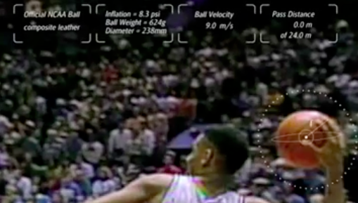
This seems like it's intended to be the initial velocity, but the ball in the frame doesn't seem to be moving yet. Known so far:
- Ball mass (incorrectly labeled weight): .624 kg
- Ball diameter: 23.8 cm (I'm not sure where this value comes from, since it actually gives a circumference that's a shade under what Wikipedia tells me is the minimum allowable under the rules)
- Initial (?) velocity: 9 meters per second
- Given that we know where the ball's going to land, they tell us that we're now at 0 of 24 meters or (presumably) horizontal distance.
This distance is a little shady to begin with. I find that the legal length for the court is 94 feet, and that the free throw line is about 19 feet off of the baseline. 24 meters puts us a yard or so inside the FT line, but Laettner's definitely on the near side of it, and he's reaching towards Hill, shortening the distance further. Perhaps this was an older standard - can someone tell me if the courts are longer now? Are they looking at the distance that the ball would've gone, had it hit the ground?
It's interesting that, using that original video and scaling the court to the foul line distance, I get just about the same distance (23.4 m vs. 24 m) that they got, without including the small bit of added distance from the fact that Hill as a little further down the baseline than Laettner was when he received the ball. It doesn't seem like this distance can be correct, given the court dimensions (the angle between the two would need to be about 22 degrees, putting Hill 9 meters down the baseline from the hoop, which isn't reasonable). Perhaps we both made the same video analysis error - checking against the court dimensions makes me think that's the issue.
The back-of-the envelope calculation for the flight is interesting. The time stops a few times during the video, but going back to original footage, I used Tracker to get a flight time of 2.069 seconds. For a distance of 24 meters, this gives a horizontal velocity of 11.6 meters per second. So much for an initial v of 9 meters per second! |
| |
 |
| |
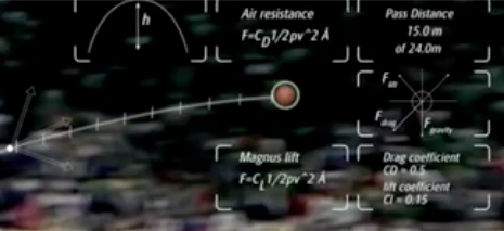
This mid-flight bit tells us that they're using a quadratic model of drag, with a drag coefficient of .5 (that seems reasonable, given some cursory internet research and the drag coefficient of a smooth sphere, though I see someone suggesting that it might be as low as .25), and a lift coefficient of .15. They're modeling the lift as being due to the Magnus force, and using the second expression from the Wikipedia description on the graphic. I saw the first in school, and I'm not clear as to whether these are equivalent or not - anyone help me out here? In any event, this effect's likely to be small, so we'll omit it from our analysis. I can model the drag part with Interactive Physics, but it's not going to be too much of an effect, I think. |
| |
 |
| |
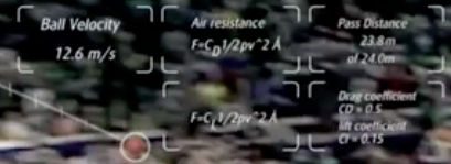
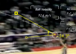
OK, in this one, the ball's very nearly there - only 20 cm to go, reportedly. They give us a velocity of 12.6 meters per second (again, if the initial velocity was 9 m/s, this isn't possible), and I get an angle of 34.3 degrees using Tracker (I tried to keep the lower line parallel to the long axis of the court - perhaps not the correct way to reference?). The angled perspective would tend to increase my measured angle, I think - correct me if I'm wrong. |
| |
 |
| |
I got an angle of about 48 degrees at the beginning, so there's certainly some perspective issue. The launch and catch heights aren't all that different, so there's considerable uncertainty in the angle measurement. Taking this 12.6 meters per second and the two angles, I get 10.4 meters per second and 8.43 meters per second as the horizontal velocities. The lower angle is closer to what I get using the original video's time, but I'm still quite suspect about the horizontal distance claimed.
Using the flight time of 2.069 s (from the original video) and assuming a .75 meter change in elevation between the beginning and the end, I get an initial vertical velocity of 10.5 m/s (10.1 m/s if you assume that there's no vertical displacement).
Combining this vertical velocity with the initial horizontal velocity from the total distance and time, I get an initial velocity of 15.6 m/s, at an angle of 42.2 degrees above the horizontal. The angle's reasonable, given my measurements and a visual inspection, but I'm not sure where the velocities given in the video come from - neither seemed to make sense.
Let's look at the motion map-like tic marks on the path: |
| |
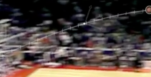 |
| |
Analyzing this first part in Logger Pro, I get a quadratic fit, though I wasn't able to get good agreement with the quadratic using the values of initial v, angle, etc.
I also extracted the x and y positions (this came from a still image, since the speed is played with during the video, so I don't know the times, though I could count all of the tic marks and calculate - I'll leave that to someone else :) ) and created a dummy time variable to graph them against (just the point number). You could check the scale again by matching up the curvature or the x-velocity, etc., but I was satisfied to see a linear x graph and a quadratic y graph: |
| |
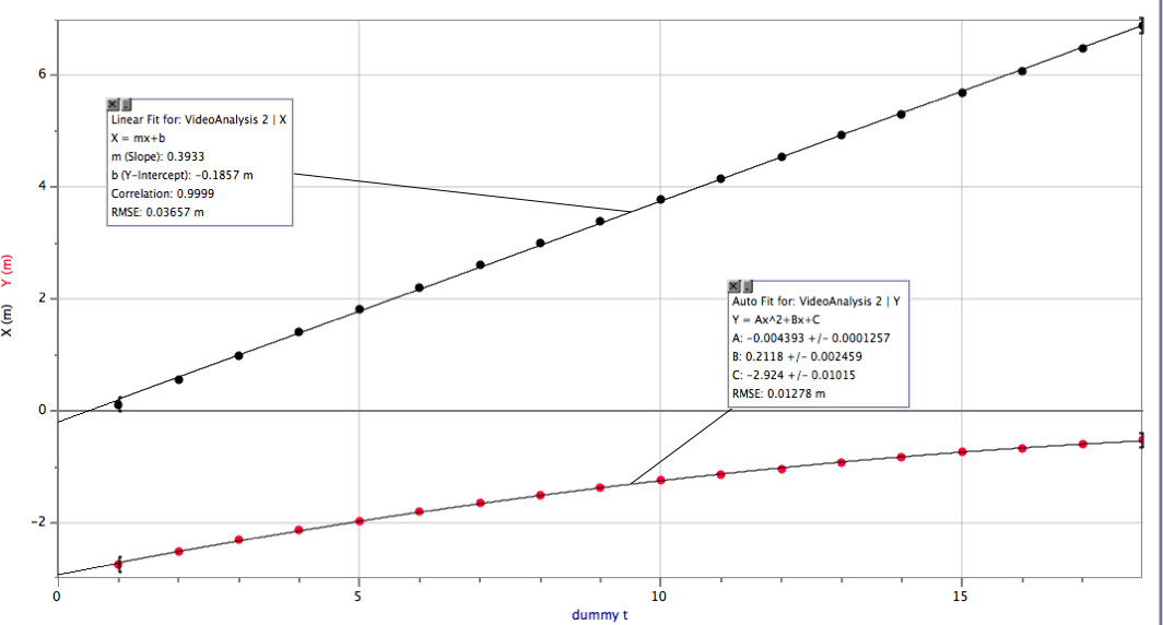 |
| |
It's a cool commercial, but there are some bits of given data that don't seem to match up with the original video and the dimensions of the court. Anyone have more analytical light to shed? Rhett?
Let me know what I've missed or miscalculated - it was a bit of a sprint during the game tonight!
Comments can be directed to Josh by Josh Gates (@DeltaGPhys), Tatnall School Willington, DE |
| |
|
| A Ceiling Fan Challenge |
| |
March 8th, 2012 by Dan Meyer
I need you to calculate the total time it will take this ceiling fan to come to a stop, and then explain your calculations. I think the keywords are "rotational kinematics" but I'm way out of my depth here. I'll call this off and post the third act (the answer) when someone gives an answer that's inside a 10% margin, paired with an explanation. The winner gets the keys to my heart.
Here's a video that (I hope) will simplify your analysis. [download] |
| |
|
| |
http://vimeo.com/38165784 |
| |
Ceiling Fan — Act Two from Dan Meyer on Vimeo.
BTW: Let's get a few guesses in there also. Totally from the gut, informed by experience only. I'm interested to see who gets closer — the analysts or the guessers.
BTW: Don't hesitate to get your students in on this also.
BTW: Yes, I already gave this a try but I was undone by the fact that I gave both the first and third act in advance which led to a lot of hand waving and glossy explanation.
2011 Mar 9. Frank Noschese gets inside the 10% envelope. His explanation, screencast, and Python script. Here's the answer video, also.
|
| Balancing Brooms: It's Not About the Planets |
| |
March
7, 2012 from Dot Physics by Rhett Allain (@rjallain)
|
| |
This isn’t new, but it is popular. Balancing a broom on its brushes. Cool trick, but the big problem is what people say.
“Hey, today is special because the planets are aligned and you can balance a broom!”
Well, today may indeed be special (it could be your birthday or something) but the position of the planets really have no effect on stuff.
One more note. I am almost certain that others have shown very similar calculations to what I will show. However, I just can’t remember where. If I had to guess, I would say it was Ethan at Starts With a Bang. But all of this has happened before and all of it will happen again. |
 |
|
| |
Gravity |
| |
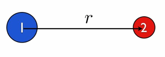
Let me start with gravity. Not your dad’s “mass times g” gravity, no the REAL stuff. Newton’s gravity (unless your dad was Newton, then these two are the same thing). Gravity is an interaction between objects with the property mass. It is not just an interaction between things and the Earth. That just happens to be the thing with the most obvious interaction. Suppose I have two objects, mass 1 and mass 2 that are separated by a distance r(as measured from the centers of the objects). |
| |
 |
| |
The magnitude of the gravitational force between these two would be: |
| |
 |
| |
Where M1 and m2 are the masses of the two objects and G is the gravitational constant with a value of 6.67 x 10⁻¹¹ N*m2/kg2. Yes, both masses have the same forces on them because forces are an interaction between two objects. |
| |
Some Sample Calculations |
| |
Let me look at the broom and estimate its mass at around 1 kg. What objects could be interacting with this broom? Well, obviously the Earth. The Earth has a mass of 5.97 x 1024 kg and the broom is 6.38 x 10⁶meters from the center (the radius of the Earth). Using these values, the gravitational force on the broom from the Earth is: |
| |
 |
| |
You know why that looks the same as your “mass times g” formula? Because it is. Where do you think g = 9.8 N/kg comes from? Now, how about a couple of planets? Right now, Venus is fairly bright in the night sky. But how far away is it? This is a perfect job for WolframAlpha. It says the distance to Venus is 1.292 x 10¹¹ meters. Since Venus has a mass of 4.87 x 1024, this means the magnitude of the gravitational force on the broom will be 1.94 x 10⁻⁸ Newtons. This force is tiny compared to the gravitational force from the Earth. Why? Because the mass of Venus is around the same mass of the Earth, but its center is WAY farther away. Ok, how about a planet with a little more mass. What about Jupiter? It has a mass of 1.90 x 1027 kg and is currently 8.29 x 10¹¹ meters away. This will create a gravitational force of 1.8 x 10⁻⁷ Newtons – still tiny. One more object. What is the gravitational force between YOU and the broom? Let’s say you have a mass of 65 kg with a distance of maybe 0.3 meters between your centers. This would create a gravitational force of 4.8 x 10⁻⁸Newtons. Yes, this is also tiny. But look, the gravitational force from you is greater than the gravitational force from Venus. So, here is your answer. How could the alignment of the planets matter when there are people around the broom that could matter almost as much (or maybe more)?
|
| |
Then How Do You Balance a Broom?
|
| |
It isn’t difficult. Really, there are two important things. First, the center of mass of a broom is quite low. Much closer to the ground than many people would estimate. Since the “brushes” part is at the bottom and bigger than the handle, the center of mass is low. Here is a picture of me with my hands at the center of mass for a broom. |
| |
 |
| |
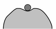
As a quick note, finding the center of mass for objects like broom is quite fun and simple. Here is a demo of how you can do that. What does the center of mass have to do with balancing a broom? Well, if the center of mass for the broom is not directly over some part of the support for the broom, it will fall over. In this case, the support area of the broom is covered by the brushes. There is another thing that is probably important. The brushes bend and act like a springy-type restoring force. This means that you don’t EXACTLY have to get the thing balanced before you let go. You just have to be close. Let describe a similar situation. Suppose you have a completely spherical bowl turned upside down. Try to balance a marble on the top of this inverted bowl and you will find it quite difficult. I guess theoretically, it is possible – but it will be tough. Now imagine a marble on top of an inverted bowl that looks like this: |
| |
 |
| |
I know, not my best drawing. Sorry, I will try better in the future. But here you can see that there are several places you can put this marble such that it will stay near the top. Of course, you can’t put it just anywhere. The broom is sort of like this. That is why it can stay up. I guess the next thing would be for me to plot the restoring force on the broom as a function of angle. Maybe someday. |
| |
 |
Rhett Allain is an Associate Professor of
Physics at Southeastern Louisiana University. He enjoys teaching and talking
about physics. Sometimes he takes things apart and can't put them back
together.
Follow @rjallain on
Twitter. |
|
| Force Vector Addition Diagrams (or, Components No More!) |
| |
March 8, 2012 from Physics! Blog by Kelly O’Shea (@kellyoshea)
The graphical solution bug has really gotten me this year (and in the best possible way). I’ve apparently done such a good job of pushing the graphical solutions that one of my classes stopped me in my tracks while I was showing them how to solve force problems by breaking the forces into components and doing 2 perpendicular N2L analyses.
“Why can’t we just use the vector addition diagram that we already drew?”
“Yeah! We can figure out how long that side is, and then we can figure out how big the gap must be. It’s not that hard.”
Not that hard? This skill (solving 2-D force problems, especially when the forces are unbalanced) has typically been one of the most difficult in the entire year of regular Physics! classes (high school juniors, typically in Precalculus) even though it wasn’t (and isn’t) any kind of big deal in the Honors Physics classes (high school sophomores and juniors, typically in Algebra 2 Honors or beyond).
So when we first start looking at unbalanced force problems and my regular Physics! students tell me to chill out because they already see an obvious way to solve them, who am I to intervene? |
|
What are Force Vector Addition Diagrams? |
| |
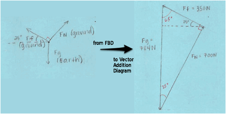
Force vector addition diagrams (a lot of students end up writing “VAD”, though I never do that) take the free body diagram (FBD) and add up all of the forces as vectors (so, head-to-tail with the size and direction of each arrow being very important). If the forces are balanced, then you should end up with nothing left over when you add them all together (). That is, when you add all of the forces together, you should end up back at the same spot where you started. So with balanced forces, the vector addition diagram is a closed shape. |
| |
 |
| |
If the forces are unbalanced, there will be a gap in the diagram since the vectors will not add up to zero. The size of the gap represents how unbalanced the forces are. The direction of the gap represents the direction of the acceleration (same as the direction of the net force). We generally draw the net force vector as a bigger, outlined arrow to distinguish it from the forces acting on the object. |
| |
 |
| |
The order of addition doesn’t matter (just as in “normal” addition). So there can be multiple correct answers to the addition problem that (to the kids) don’t look the same as each other. The result will look the same, but the shape created by the vectors might look different. Some students have understood that for a while and some are just starting to realize the subtleties there. |
| |
|
| |
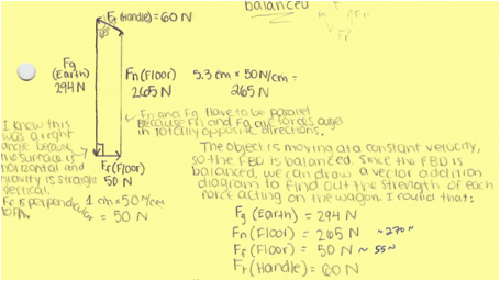
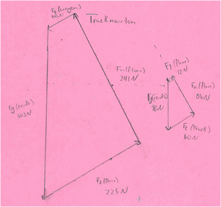
Both of those diagrams show correct vector additions from the same correct FBDs (the second one had some trouble with the numbers, but the shape was correct).
|
| |
Break out the Protractors: Using Vector Addition Diagrams to Solve Problems |
| |
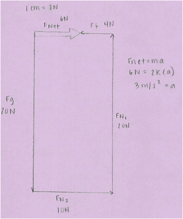
At first, we always draw the diagrams to scale. As long as you know enough about the directions and/or lengths of the vectors, you can figure out the direction(s) and/or length(s) that you don’t know.
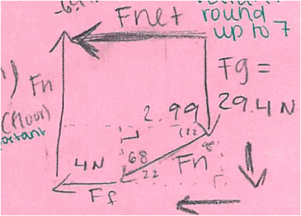
Here’s a great student solution from a quiz. It was early on in our experience with vector addition diagram drawing, so she wrote a lot of her thoughts out as she talked herself through how to set up her work. In light pencil marks near the top (right-ish), you can see the sketch of the general shape she did before trying to draw it to scale. She writes out her conversions between her measurements in centimeters and the values in newtons.
|
| |
 |
| |
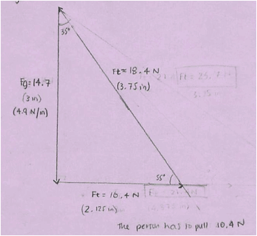
Drawing the diagram (especially to scale) can help struggling students check to see whether their answers make sense. |
| |
 |
| |
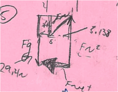
You can see the erased lines from previous attempts at solving the problem. Once she had drawn the angles, she realized that there must have been something wrong with what she had done. She persisted in figuring out what was wrong until her entire solution was correct.
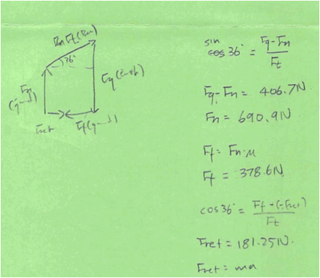
As they became more comfortable with the diagrams, many students started drawing just the sketch, labeling the angles, breaking the shape into smaller shapes (triangles, rectangles) and using right angle trigonometry to find the unknown lengths and directions. They saw the opportunity to use trig without my suggesting it to them and while they already had another, perfectly valid, way of solving the problem. I like that so much better than feeding them components while I teach them an algorithm. |
| |
 |
| |
Some students (especially the juniors in Algebra 2) haven’t learned about sine/cosine/etc yet. It would be easy enough to just show them how to use the button on the calculator, but they are (so far) more than happy to keep using the protractor and a scale drawing to solve problems. They already have a method that makes total sense to them. |
| |
 |
| |
Now that we are in the new semester and two units (soon to be three) removed from when we learned about unbalanced forces, I’m starting to see a few students “invent” the idea of looking at the x- and y-components of the forces and doing a Newton’s 2nd Law analysis in component form. After spending so much time with the vector addition diagrams, they started to see the pattern about finding the size of the horizontal sides and the size of the vertical sides in pretty much any diagram they drew.
Using these diagrams as an “exclusive” (until they figure out otherwise) way of solving force problems has been great for my students this year. Compared to past years, many many more of them find success in situations with unbalanced forces and the level of understanding (for all students, including the strongest ones) is deeper. Using one of these diagrams to solve a problem shows much more understanding about how the quantities are related than does churning through an algorithm and writing down a lot of equations. So, win-win.
|
| Polarized Light Demo |
| |
By Tony Wayne
Materials:
Light source, glass, polarizer film, paper
Procedure:
Write a secret message on the paper. Something like, “Go Patriots!” or “Only geniuses can see this.” Create the setup shown below. If the angle is right, the glare from the light will hide the message when viewed by the naked eye, or camera. Hold the plastic polarizer between the eye and glass as shown. When rotated to the correct position, the glare will be blocked and the message can be viewed.
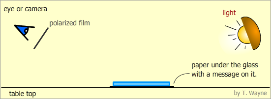
Presentation:
I like to use this at the beginning of a class (on a day when we will be discussing polarization) and I do not explain any of the physics behind it. Instead I challenge the students to describe what happened by the end of class. At some point during class enough hints and pieces may be given for them to figure out what is happening.
The Physics:
When light is bounced off a surface, a majority of the electric field component of the light is parallel to the surface. When the polarizer is rotated perpendicular to the plane of the glass, the glare is greatly reduced or eliminated and the message underneath can be read. This could lead to a conversation about Brewster’s angle.
Brewster’s angle is the angle where the maximum amount of reflected light is polarized. This angle is found from
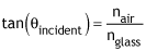
In the case above, θincident is angle the incident light makes with the normal line to the surface, (not pictured,) “n” represents the indices for air and the glass the light bounces off of. |
| |
|
| |
|
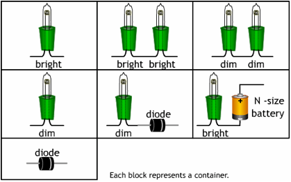
| Mystery Circuit Box Activity |
| |
| Presenter: Tony Wayne, twayne@k12albemarle.org, Albemarle High School |
Va. SOL:
PH.3 The student will investigate and demonstrate an understanding of the nature of science, scientific reasoning and logic.
PH.11 The student will investigate and understand how to diagram, construct, and analyze basic electrical circuits and explain the function of various circuit components. Key concepts include:
a) Ohm’s law; b) series, parallel, and combined circuits
National Standards:
http://www.nap.edu/readingroom/books/nses/html/6e.html#ps
Topic/Concept
Student create a tool to be used to investigate simple, mystery, circuits.
Materials
- A string of 20 Christmas light bulbs that plug into a 120 V outlet
- A string of 50 or 100 Christmas light bulbs that plus into a 120 V outlet.
- 7 or more small jewelry boxes or 35 mm film canisters, or something similar that is light tight. You could use toilet paper tubes with the ends closed off.
- 1 “N” size alkaline battery
- 2 “AA,” alkaline, batteries. (At least 2 per student group.)
Safety Considerations
Warn student what a short is how quickly the wire gets hot enough to burn. Also describe to the students that if it gets hot, LET GO! It amazes me how many students want to hold on to a hot wire.
Presentation
Before doing this activity, I like to do an introductory activity similar to http://vip.vast.org/NSTA/circuit/default.htm
In a previous activity student divided light bulb up based up brightness and learned about what a diode does to the current in a circuit. They are again provided with those same pieces but it is up to the student to choose what they want. Below are the suggested contents for the boxes.
|
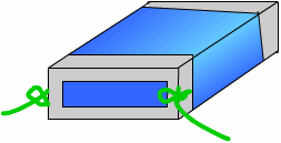
Example Box
|
When the box/container is closed, tape is closed to keep prying eyes out. Make sure stripped wires are poking out of the box. Tie knots in the wires outside of the boxes to keep the wires from receding back into the box.
How the physics is demonstrated
The specifics depend on which mystery box the student chooses. It is as much logic problem as anything else. What a student should do is to come up with a series of tests and carry them out to figure out what is in each mystery box.
Construction and Tips Regarding the Demonstration
I use Christmas lights because they are cheaper than the typical “long” and “short” bulbs that are used with the CASTLE method of teaching electricity. The two strings of bulbs use bulb with different resistances. |
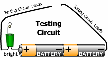 |
The testing circuit can The extra battery will make it easier to see changes in the brightness of the light bulb,
To test for a diode, use a battery, a diode and bright bulb. The bright bulb is used so if it burns dimly, it can still be seen. Touch the test circuit to the leads of the mystery box and then reverse the lead. If there is a diode in the circuit, the test will light up in one direction and not in the other direction. The box with the battery will look very similar to the one with a light and diode. But the brightness will be brighter.
Sometimes I make this box the challenge box and not part of the typical discovery process because of its trickiness.
Sources & References
None |
| Bringing Computational Modeling into First Year high School Physics |
| |
June 14, 2011 From Quantum Progress, by John Burk (@occam98)
I’ve previously written quite a bit about the wonders of computational modeling and the great things Danny Caballero and his colleagues at Georgia Tech have done to create an awesome set of tools to make using creating and using computational models in physics easier and more powerful.
In this post, I’m going to share how I’m trying to create a series of lessons and assessments that tightly weave computational modeling into the 9th grade modeling physics curriculum I teach.
First, let me outline my goals:
- I want students to see computational modeling as a fifth tool for understanding a physical system. I want them to think that they can describe a system verbally, mathematically, graphically, diagrammatically, and now with a computational model. I want them to see the links between these models, the power the computer has to help them to visualize them.
- I want my students to see the power of computational modeling to explore systems that cannot be explored by other means. I want them to see how easy it is to add air resistance to the motion of a soccer ball, or imagine what would happen to the motion of the planets if the gravitational force were an inverse cube law.
- I want my students to see overall paradigm of computational modeling as an extension of the power of Newton’s laws. We can predict the future by simulating the motion of the object over very tiny steps as constant velocity, and then updating the velocity using the forces acting on the object. In this way, I want them to see that all of their programs, different as they may look, share this common feature.
- I want to do my part to create enthusiastic programmers that have an appreciation for computer science and a understanding good coding practices.
To accomplish these goals, I am going to try to develop a series of activities for each unit that introduce programming gradually, trying to reinforce and expand the current model they are studying (e.g.. Constant velocity, or Simple Harmonic Motion). We’ll begin by having them make physical measurements from models that have already been created for them, and move to having students modify the code of the models to change the simulations. As students progress and get a better understanding of how to write good code, they will develop their own models from scratch.
Here’s the first lesson I’ve put together. If you’re interested, I’d love for you to give it a whirl.
- You should start by following the instructions at vpython.org to download and install vpython.
- Next, download the zip archive of the necessary files. This contains the 1-dMotionSimulation.py program we’ll be working with, as well as the PhysUtil python module created by Georgia Tech.
Finally, I’ve created this short 3 minute introduction that explains how to open and run the 1-d Motion Simulation, and lays out the first challenge: finding the velocity of the ball 3 different ways, and then changing the program so that the ball starts on the right side of the field and moves to the left. I would imagine that this first assignment would take most of my students somewhere around half an hour to do, starting from scratch, with no previous exposure to programming.
The video: http://vimeo.com/25070908
This video isn’t meant to be a Khan-like expose fully explaining all the details of vpython. Instead, I wanted it to be a short introduction that got three main ideas across:
- Reading comments is critical to understanding.
- Understand the overall structure of the program and how it’s broken down into parts.
- You can figure this out by exploring. Here are three chords—go start a band.
Ultimately, I’ll code this challenge up as a Webassign assignment, but I wanted to put this out now to share with you for feedback.
|
| Three Great Links |
| |
1. Physics! Blog! by Kelly O'Shea http://kellyoshea.wordpress.com
2. Noschese 180, A picture-a-day for the school year by Frank Noschese http://noschese180.posterous.com
3. 101 Questions by Dan Meyer http://101qs.com
"Dear Ms./Mr./Dr. _____________,
We don't care how well you lecture. We don't care how well you engage us. We aren't impressed by your fancy slide transitions or your interactive whiteboard. We care how well you perplex us.
Can you perplex us? Can you show us something that'll make us wonder a question so intensely we'll do anything to figure out the answer, including listen to your lecture or watch your slides? Here's one way to find out. Upload a photo or a video. Find out how many of us get bored and skip it. Find out how many of us get perplexed and ask a question
Then figure out what you're going to do to help us answer it.
Signed,
Your Students" |
| Opportunities for PhysicsTeachers |
| |
VAST Mini-Grant |
| |
Need funding for an innovative curriculum activity? VAST's minigrant application for funding is due June 1. The application is short and can be found here:
|
| |
Professional Development |
| |
Matter and Interactions Distance Education Course:
|
| |
Modeling Instruction in High School Physics Workshop:
|
| |
NSTA 2012 Area Conferences
- Louisville, Kentucky: October 18–20
- Atlanta, Georgia: November 1–3
- Phoenix, Arizona: December 6–8
|
| |
"Science of Nuclear Energy & Radiation" 2012 4-DAY Science Teacher Workshop:
|
| |
|
| |
Nanoscience: The Big Ideas of Nanoscience and Nanotechnology August 1-3; 6-10
|
| |
Innovations in Inquiry3 , June 21 and 22, 2012
|
| |
UVA Professional Development Opportunities in Physics Education
|
| |
Virginia Association of Science Teachers Profession Development Institute (VAST-PDI)
|
| |
AAPT Summer Meeting: Philadelphia, July 28 –August 1 2012
|
| |
Virginia Association of Science Teachers
(VAST)

|
American Association of Physics Teachers
(AAPT)

|
American Modeling Teachers Association (AMTA)

|
National Science Teachers Association (NSTA)

|
|
| Are You on our E-mail List? |
| |
If you have any physics-related questions, news, or anything else? Please post it to the yahoogroup (http://groups.yahoo.com/group/va-inst-phys/) or send it to us directly. |
| |
|
| |
|
|